Welcome to my first installment of comprehensive examination hell. Don’t worry, it may actually be fun. Today, I’ll be giving a basic intro to the Holling “Disc” equations and how well they may or may not describe the relationship between grey seals and cod on the east coast. There are two ways to read this post: You can jump over the mathematical proofs and jump right to an easy explanation of how different modeling approaches impact your view of the grey seal cod issue. It is my belief that most explanations to date are inaccessible to the non-science crowd, and that doesn’t seem fair. If you want to skip to implications, you can start reading after the graphic near the bottom. If you prefer to relive all the grisly modeling details with me, then keep reading. Choose wisely.
It is important to remember that there are several fundamental assumptions built into these “models of reality” and we may or may not have reasons to justify these assumptions. Functional feeding responses don’t necessarily help to describe other issues, like the prevalence of seal worm in cod fillets, but they can imply circumstantial connections. Predator-Prey models simply address one part of the world–a building block that needs to be in context to understand its full implications. The non-math people can stop here if they wish.
In C.S. Hollings’ early work, he designed a very simple and intuitive experiment. He blindfolded a group of people then asked them to search for sandpaper “discs” that he placed at random on a smooth floor. He discovered that early on in the experiment, the poor blindfolded souls did a reasonable job of finding the discs. As time wore on, the subjects spent more time “searching” for discs simply because there were fewer available to be found. He developed a very simple equation to describe this phenomenon:
Tt = Ts + Th
where Tt was the total time spent “foraging” or engaging in seeking out discs, Ts was the time spent in active search, and Th was the time needed to physically pick up or “handle” the discs. From this simple equation, we can derive three different functions based on different lines of logic. These, Holling “Disc” equations describe different types of predator prey interactions that require different assumptions to analytically solve. Here’s the Type I:
Type I Assumptions: Handling time and search time are negligible. We know this to be rare in nature and is more commonly a situation that arises in laboratory experiments (more on this later). We can simply describe Type I as:
NE = mNo
where NE is the number of prey eaten by the predator and is proportional to prey density/abundance only up to some maximum (when predators can eat no more).
Type II Assumptions: predators eventually become “satiated,” but in this case, it is because the predator becomes limited by the time spent “handling” the prey. We can start with Hollings’ original time budget equation:
Tt= Th+ Ts
Now, we can express handling time as:
Th=hNE
where h is the time lost to handling and NE is the number of prey eaten. Next we can express the number of prey eaten, NE as:
NE=aTsN0
where a is some “rate of attack” and N_0 is the total density or abundance the prey. Substituting NE into the time budget equation:
Tt=ahTsN0+ Ts which is the same as:
Tt= Ts (1+ahN0) when expressed in terms of Ts, it becomes:
Ts=Tt/((1+ahN0))
And finally, substituting this into the equation for NE:
NE=(ahTt N0)/((1+ahN0))
And Voila! We have a Hollings Type II equation.
Type III Assumptions: As in the Type II equation, predators become “satiated” but at low prey densities/abundances, the time spent searching (T_s) increases as prey become harder to find and encounter rates become lower. To graphically display this behavior, we simply square the denominator:
NE= (ahTt N0)/((〖1+ahN0)〗^2 )
Here is what we can expect to see graphically from the Type I, II, and III equations:
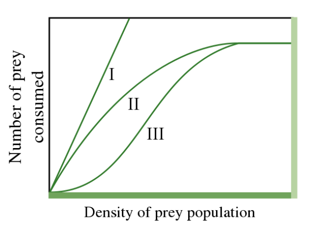
Photo Credit: Wikimedia Commons
Now back to cod and grey seals. We can exclude the Type I equation. We know from natural experiments that handling time and search time are extremely important considerations. That leaves us with two views of the cod and grey seal world.
The argument for a TYPE II response
The first view, a Type II has serious implications for a severely depleted cod stock. Referencing the graph above, a Type II response suggests that grey seals could potentially consume cod to near extinction. That means that cod as a population either, a) have no habitat refuges (hiding spots) to escape grey seal predation so as to reduce encounter rates (increase searching time), or b) cod do have refuges but their life history is such that they aggregate so that they are easily found or grey seals have learned to find them when they aggregate. There is support for b) because cod aggregate to spawn in the summer months, making them far more vulnerable than at other times of the year. Cod may be doubly vulnerable in areas where past trawling activity has destroyed bottom cover.
The argument for a TYPE III response
There is the general belief among many (scientists and non-scientists alike), that depletion of fish populations is unnatural and only happens in response to fishing pressure. In fact, this isn’t always the case. Some fish life histories are such that their populations may crash in response to factors such as El Niňo. These stocks have evolved to sustain these periodic crashes by having high rates of production when environmental conditions are favorable again. In these cases, fish populations may have evolved to sustain periodically high predation rates. Fish often rely on refuges to hide from predators. The predators, in turn, experience low encounter rates with prey. There tends to be an increase in search time and handling time as predators have less and less experience efficiently handling prey. If we reference the graph about, this results in the characteristic “inflection” at low prey densities, where consumption rates are nearly zero due to lower encounter rates.
When we see a curve such as this, it could suggest that predators need to engage in active “prey switching” in order to survive. This may be what we are seeing today in the Gulf of St. Lawrence. Grey seals are encountered with increasing frequency by fishermen engaging in fisheries other than depleted groundfish species. Herring and mackerel fishermen report grey seal “herding” behavior to feed on shoals. This is possibly a response related to learning a new “handling” strategy because the encounter rates with herring are now much higher than they are for cod and other groundfish.
The modeling to date suggests that a Type II response for cod and grey seals for the Eastern Scotian Shelf. However, the key weakness in these studies has been a lack of agreement between the grey seal diet information and a Type II feeding response. How does this happen?
Because we essentially use two different methods to assess the feeding response and grey seal diet. Due to the incompleteness of the diet data, functional feeding responses are built around results from stock assessment modeling which provides detailed information on natural mortality rates. Operating on a different set of assumptions (which I will not go into here), modelers can estimate cod mortality attributed to grey seals. This information can help us make inferences about grey seal consumption that can be quite robust IF we can rely on the inherent assumptions of those models. Conversely, the dearth of long-term and more importantly spatially representative diet data from grey seals do not allow us to “ground-truth” functional feeding response models. Consequently, the problem becomes circular, and we are reduced to relying on assumptions about diet. Whether right are wrong, these diet assumptions remain the most contentious and divisive issue among scientists.


